Physics Lab Notes

Below are short concept notes connected to Experiments 2–5
(Directed motion, Random motion, Random + directed motion, and Vesicle transport).

Experiment 2 – Directed motion (Terminal velocity)

In the coming weeks, your main lecture will cover terminal velocity and the role of resistive forces. To help you get a head start, here is a short introduction that outlines the basic concepts and includes a few equations showing how terminal velocity depends on various parameters.

This document is meant to give you a general idea. Your own predictions about parameter dependence may differ, and your experimental results might not match the theory exactly.

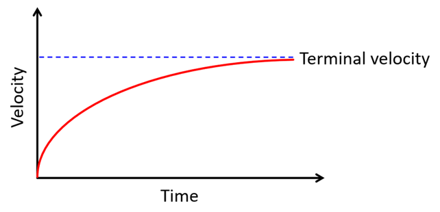
Terminal velocity

When an object falls through a fluid (air, water, glycerin, etc.), several forces are at play. When you release the sphere, it falls toward the ground (toward the center of the Earth, to be more precise). This is due to the force of gravity, i.e., its weight. But since it is moving through a fluid (not a vacuum), it also experiences a resistive force that tries to slow the object down, much like friction.

So we have a downward gravitational force and upward resistive forces on the object. The resistive force depends on the velocity of the object, so it increases as the object accelerates. The downward gravitational force, however, remains the same. At some point, these forces balance out, making the net force zero, i.e., acceleration zero, which means the velocity becomes constant. This constant velocity is called the terminal velocity.

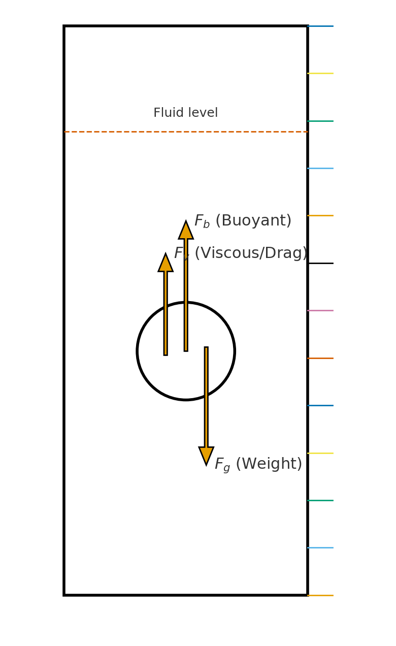
Velocity vs time for object reaching terminal velocity

Forces on a falling sphere

For a sphere of radius (r), density (\rho_s), and mass (m) falling through a fluid of density (\rho_f) and viscosity (\eta):

Weight (downward)

[ F_g = mg = \rho_s V g ]

where (V = \tfrac{4}{3}\pi r^3) is the volume of the sphere.
Buoyant force (upward, Archimedes’ principle)

[ F_b = \rho_f V g ]
Velocity-dependent resistive forces (drag forces, upward)

At low speeds and for small spheres, viscosity dominates and Stokes’ law applies:

[ F_v = 6\pi \eta r v ]

At higher speeds / turbulent flow, drag depends on velocity squared:

[ F_d = \tfrac{1}{2} C_d \rho_f A v^2 ]

where (A = \pi r^2) is the cross-sectional area of the sphere and (C_d) is the drag coefficient.

For the current experiment, we can neglect the turbulent contribution and only consider the viscous force.

Condition for terminal velocity

At terminal velocity (v_t), the net force is zero:

[ \text{Total downward force} = \text{Total upward force} ]

[ F_g = F_b + F_v ]

Substituting:

[ \rho_s V g = \rho_f V g + 6\pi \eta r v_t ]

Solving for (v_t):

[ v_t = \frac{(\rho_s - \rho_f) V g}{6\pi r \eta} = \frac{2 r^2 g (\rho_s - \rho_f)}{9 \eta} ]

Terminal velocity

[ v_t = \frac{2 r^2 g (\rho_s - \rho_f)}{9 \eta} ]

where
(r) – radius of the sphere
(g) – acceleration due to gravity (\left(9.8\ \text{m/s}^2\right))
(\rho_s) – density of the sphere
(\rho_f) – density of the fluid
(\eta) – coefficient of viscosity

Our experiment investigates the dependence of (v_t) on

the size of the sphere, (r)
the density of the sphere, (\rho_s)
the viscosity of the fluid, (\eta)

Qualitative predictions:

(v_t) vs radius (r) – parabolic (\left(v_t \propto r^2\right))
(v_t) vs density (\rho_s) – linear (\left(v_t \propto (\rho_s - \rho_f)\right))
(v_t) vs viscosity (\eta) – inverse (\left(v_t \propto 1/\eta\right))

Experiment 3 – Random motion (Brownian motion & diffusion)

In this experiment, we look at motion on the microscopic scale, known as Brownian motion. This was one of the first clear pieces of evidence for the existence of molecules. Robert Brown noticed that pollen grains under a microscope seemed to “wiggle” around, which is due to water molecules constantly bumping into the pollen, making it move randomly.

In our class, we replicate this idea by observing tiny silica beads suspended in water under a microscope. We then study how the random motion (or diffusion) of these beads depends on two things: the radius of the bead and the viscosity of the liquid they are in.

Root mean square (RMS) distance

Consider placing a drop of ink gently on the surface of water in a test tube (to minimize convection and other disturbances) and starting your clock. At time zero, the ink particles are all at the starting point. As time passes, they spread out. Eventually (after many hours), the entire column of water changes color, reaching a uniform concentration of ink particles throughout.

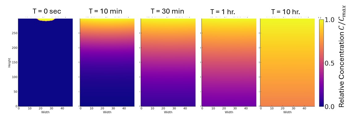
This process is called diffusion, the transfer of particles from a region of higher concentration to a region of lower concentration. Diffusion occurs due to the underlying random, or Brownian, motion of the particles.

A naive idea is to take the average displacement of all the particles from the initial point. But since diffusion is a random walk, each particle has an equal chance of moving left or right. When we add up all these displacements, they cancel out, and the average displacement is always close to zero. So the simple arithmetic mean is a poor choice.

Instead, we use the root mean square (RMS) displacement, which is a statistical mean:

Square each displacement (this removes negative signs so left and right don’t cancel).
Take the average (mean) of these squared displacements.
Take the square root to return to distance units.

RMS displacement

[ r_{\text{rms}}(t) = \sqrt{\frac{r_1^2(t) + r_2^2(t) + \dots + r_N^2(t)}{N}} ]

where
(r_i(t)) – displacement of the (i^{\text{th}}) particle at time (t)
(N) – total number of particles

For diffusive motion in 2D, the RMS distance is related to the diffusion constant by

RMS distance in 2D

[ r_{\text{rms}}(t) = \sqrt{4 D t} ]

where
(D) – diffusion constant
(t) – time

Einstein proposed that the diffusion constant depends on temperature and on the mobility, defined as

[ \mu = \frac{v}{F}, ]

which quantifies how easily an object moves under an applied force.

Einstein related diffusion to mobility through

[ D = \mu k_B T, ]

where (k_B) is Boltzmann’s constant and (T) is the absolute temperature.

During random motion in a liquid, the dominant force is viscous drag (Stokes’ law):

[ F_{\text{viscous}} = 6\pi \eta r v, ]

so the mobility is

[ \mu = \frac{v}{F_{\text{viscous}}} = \frac{1}{6\pi \eta r}. ]

Combining gives the Stokes–Einstein relation:

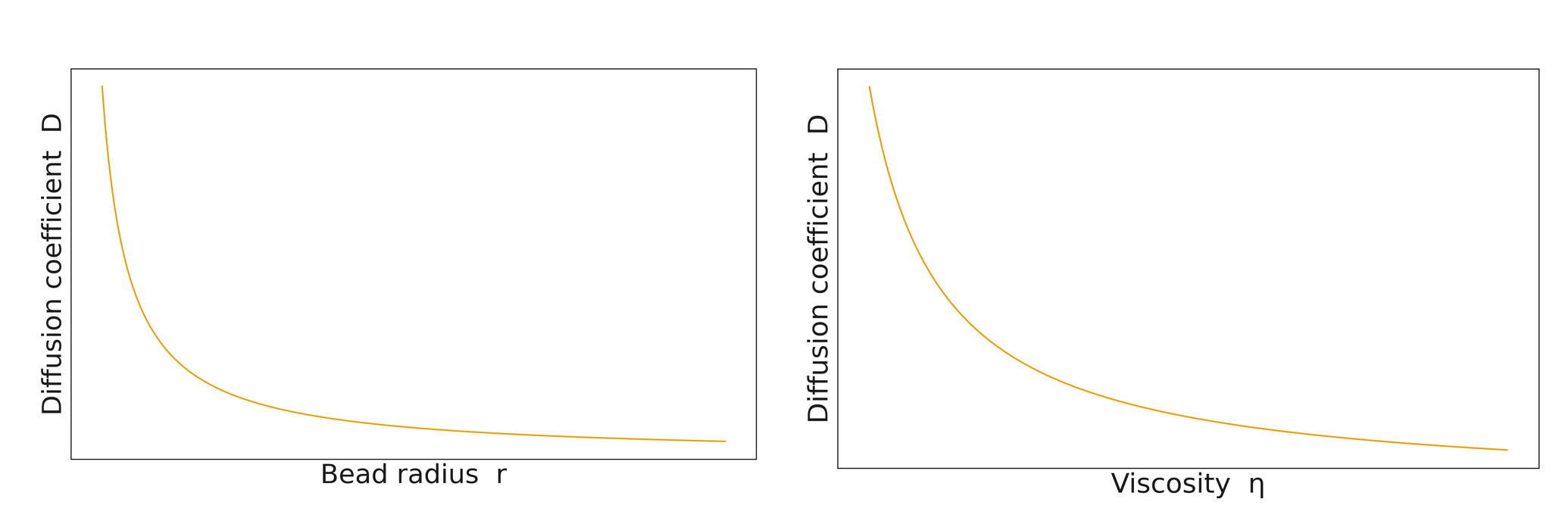
Diffusion constant (D)

[ D = \frac{k_B T}{6\pi \eta r} ]

where
(T) – temperature
(\eta) – coefficient of viscosity
(r) – radius of the spherical particle

Using ImageJ data

The aim of this experiment is to determine how bead radius and fluid viscosity affect the diffusion constant.

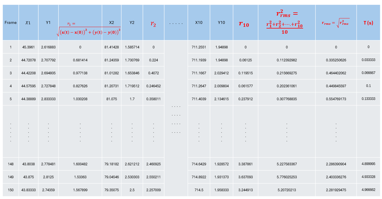
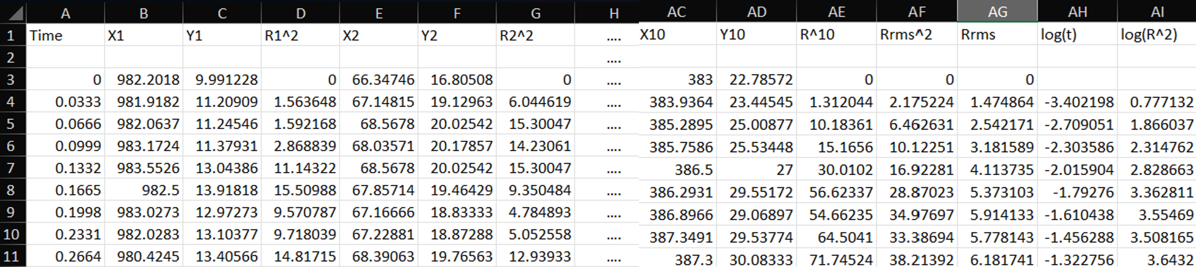
Following the lab manual, you will record three videos of beads suspended in liquid and track at least 10 particles. From the ImageJ output, you will obtain the (x) and (y) positions of the tracked particles.

Take the position at the first frame ((t=0)) as the initial position.
At each later frame, the displacement of a bead is

[ r(t) = \sqrt{(x(t) - x(0))^2 + (y(t) - y(0))^2}. ]

Then compute the squared RMS distance for each time frame:

[ r_{\text{rms}}^2(t) = \frac{r_1^2(t) + r_2^2(t) + \dots + r_{10}^2(t)}{10}. ]

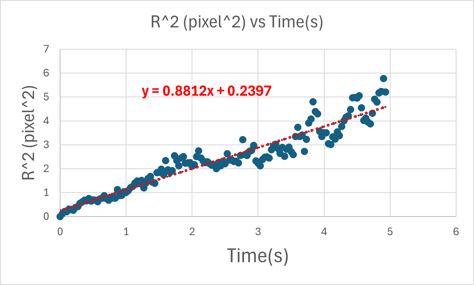
According to the 2D RMS relation,

[ r_{\text{rms}}^2 = 4 D t. ]

So if we plot (r_{\text{rms}}^2) versus time (t), the slope is (4D). Therefore,

[ D = \frac{\text{slope}}{4}. ]

Experiment 4 – Random + directed motion

In this week’s experiment, we tilt the microscope stage, introducing a gravitational force component. This adds a directed force that tends to pull the beads in one direction.

Random motion (Brownian motion) causes particles to spread out in all directions.
Directed motion (due to gravity) causes particles to drift preferentially in one direction.

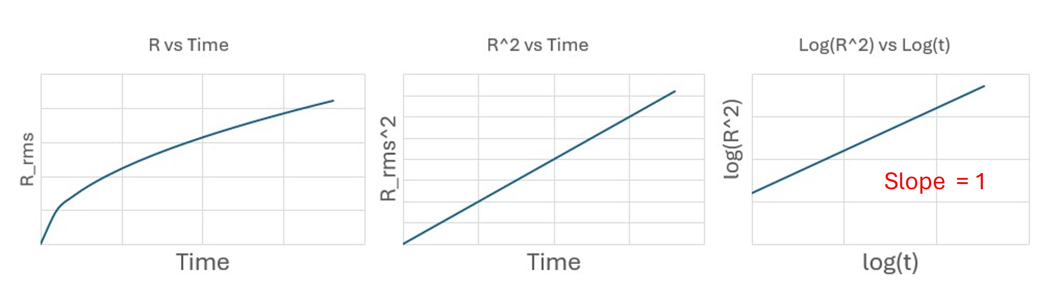
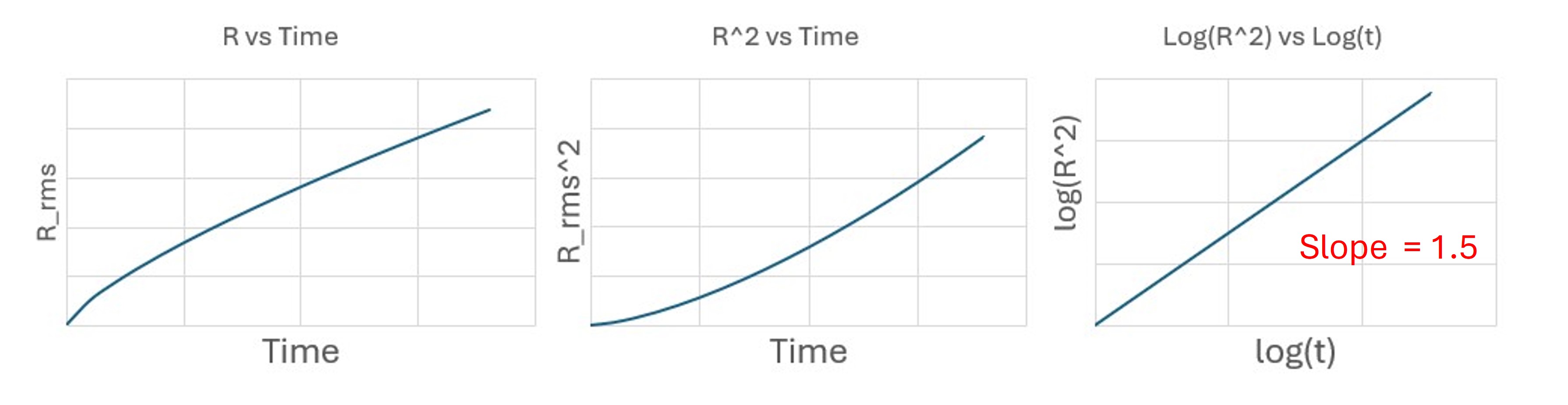
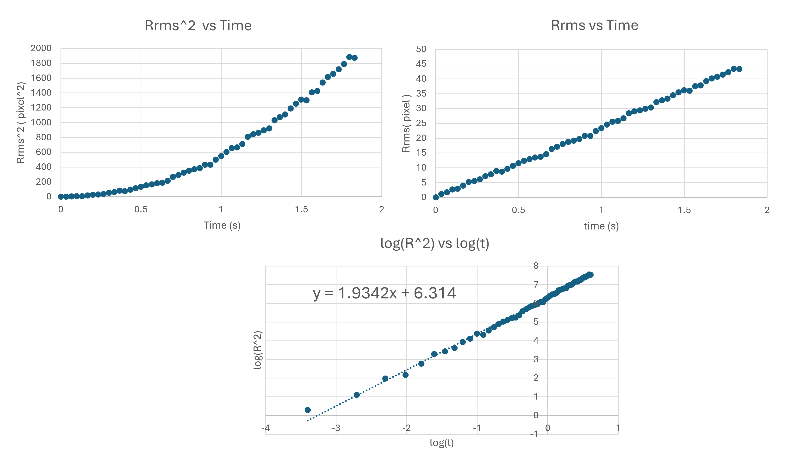
To distinguish these behaviors, we analyze bead trajectories using log–log plots of mean-squared displacement versus time.

Purely random (diffusive) motion

For Brownian motion in two dimensions:

[ R_{\text{rms}}^2 = \langle r^2(t) \rangle = 4Dt. ]

Taking logarithms:

[ \log(R_{\text{rms}}^2) = \log(4D) + \log(t). ]

So the slope on a log–log plot is

[ m = 1. ]

Diffusion-dominated motion: slope (\approx 1).

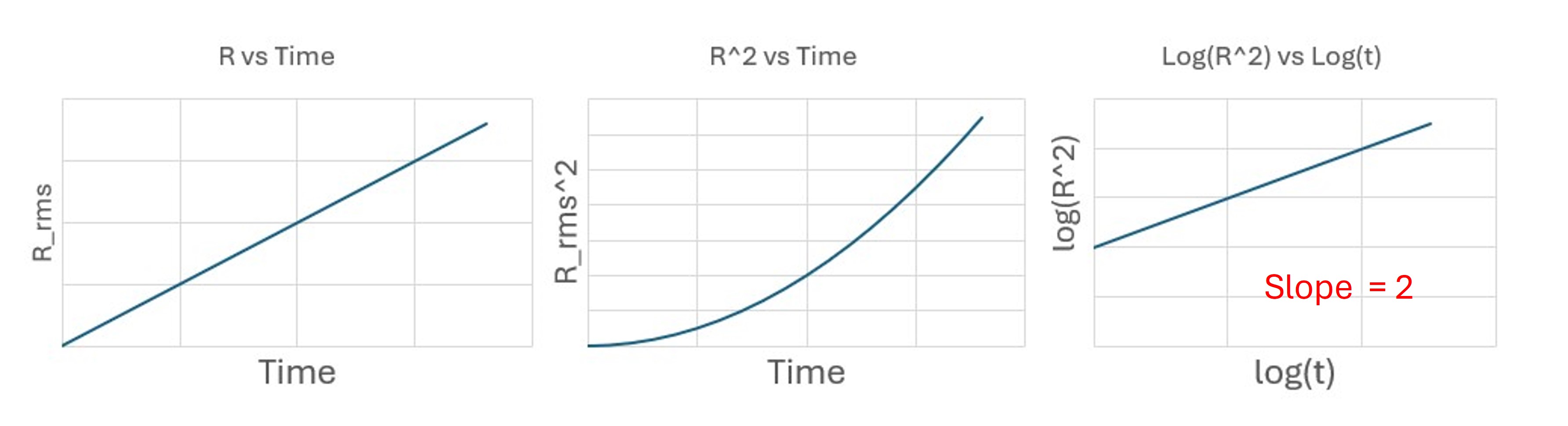
Purely directed motion

With constant drift velocity (v):

[ r(t) = vt \quad \Rightarrow \quad R_{\text{rms}}^2 = v^2 t^2. ]

Taking logarithms:

[ \log(R_{\text{rms}}^2) = \log(v^2) + 2\log(t), ]

[ m = 2. ]

Directed motion: slope (\approx 2).

Mixed motion

If both effects occur:

[ \langle r^2(t) \rangle \propto t^\alpha, ]

with (1 < \alpha < 2).

For this experiment:

(2\,\mu\text{m}) beads → slopes closer to 1
(5\,\mu\text{m}) beads → slopes closer to 2

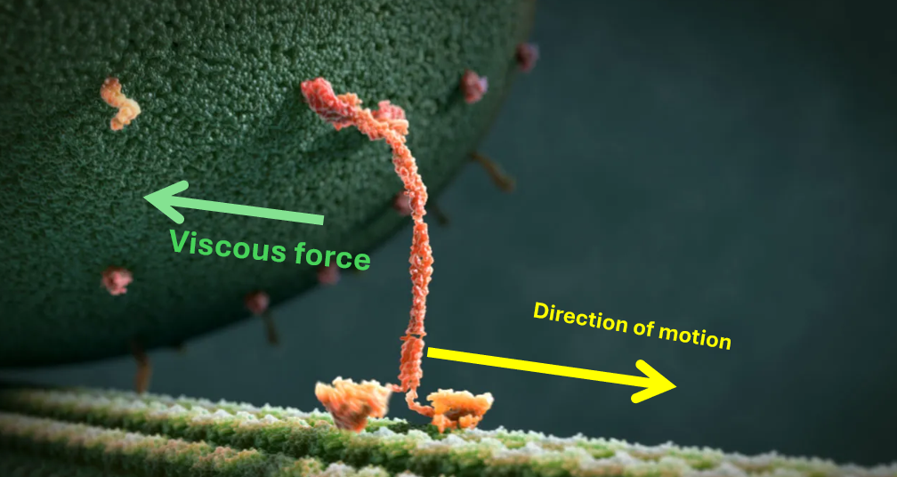
Experiment 5 – Vesicle motion, ATP hydrolysis & viscosity

To calculate the rate of ATP hydrolysis (R) and the coefficient of viscosity (\mu), you will use the average radius (r) and average speed (v) obtained from ImageJ.

Work and power

[ W = \mathbf{F} \cdot \mathbf{d} = |\mathbf{F}|\,|\mathbf{d}| \cos\theta, ]

and

[ P = \frac{W}{t}. ]

Useful biological numbers:

Kinesin step size: (s_{\text{kin}} \approx 8\,\text{nm})
Myosin step size: (s_{\text{myo}} \approx 10\,\text{nm})
Energy released per mole of ATP: (E_{\text{mol}} \approx 23\ \text{kJ/mol})
Energy per ATP molecule:

[ E = \frac{E_{\text{mol}}}{N_A} ]
Motor efficiency: (e \approx 0.6)

[ e = \frac{P_{\text{produced}}}{P_{\text{consumed}}}. ]

[ P_{\text{consumed}} = R E, \quad R = \frac{N}{t}. ]

[ P_{\text{produced}} = F v. ]

Rate of ATP hydrolysis (R)

[ v = \frac{d}{t}, \quad d = Ns \Rightarrow v = Rs. ]

[ R = \frac{v}{s}. ]

Coefficient of viscosity (\mu)

Stokes’ law:

[ F_{\text{viscous}} = 6 \pi \mu r v. ]

From efficiency:

[ e R E = F v \Rightarrow F = \frac{e R E}{v}. ]

Thus

[ \mu = \frac{F}{6\pi r v} = \frac{e R E}{6\pi r v^2}. ]

Using (R = v/s):

[ \mu = \frac{e E}{6\pi r v s}. ]

Compare with water:

[ \mu_{\text{water}} \approx 8.6 \times 10^{-4}\ \text{Pa·s}. ]